Sea Ice Thickness, Volume & Mass
Centre for Polar Observation and Modelling
Overview of the processing chain used to derive sea ice thickness and volume.
The data products provided on this portal are generated using a well-established processing chain primarily derived from CryoSat-2 radar altimeter data. The methodology summarized below is detailed comprehensively in the paper:
Estimating Arctic sea ice thickness and volume using CryoSat-2 radar altimeter data
(Tilling et al., 2018; Advances in Space Research).
The process begins by utilizing CryoSat-2 Ku-band radar altimeter data operating in SAR (Synthetic Aperture Radar) and SARIn (Interferometric SAR) modes. This high-resolution radar altimetry provides the fundamental echo waveforms measured over the polar oceans. These data are available from ESA's CryoSat L1b Baseline-E archive.
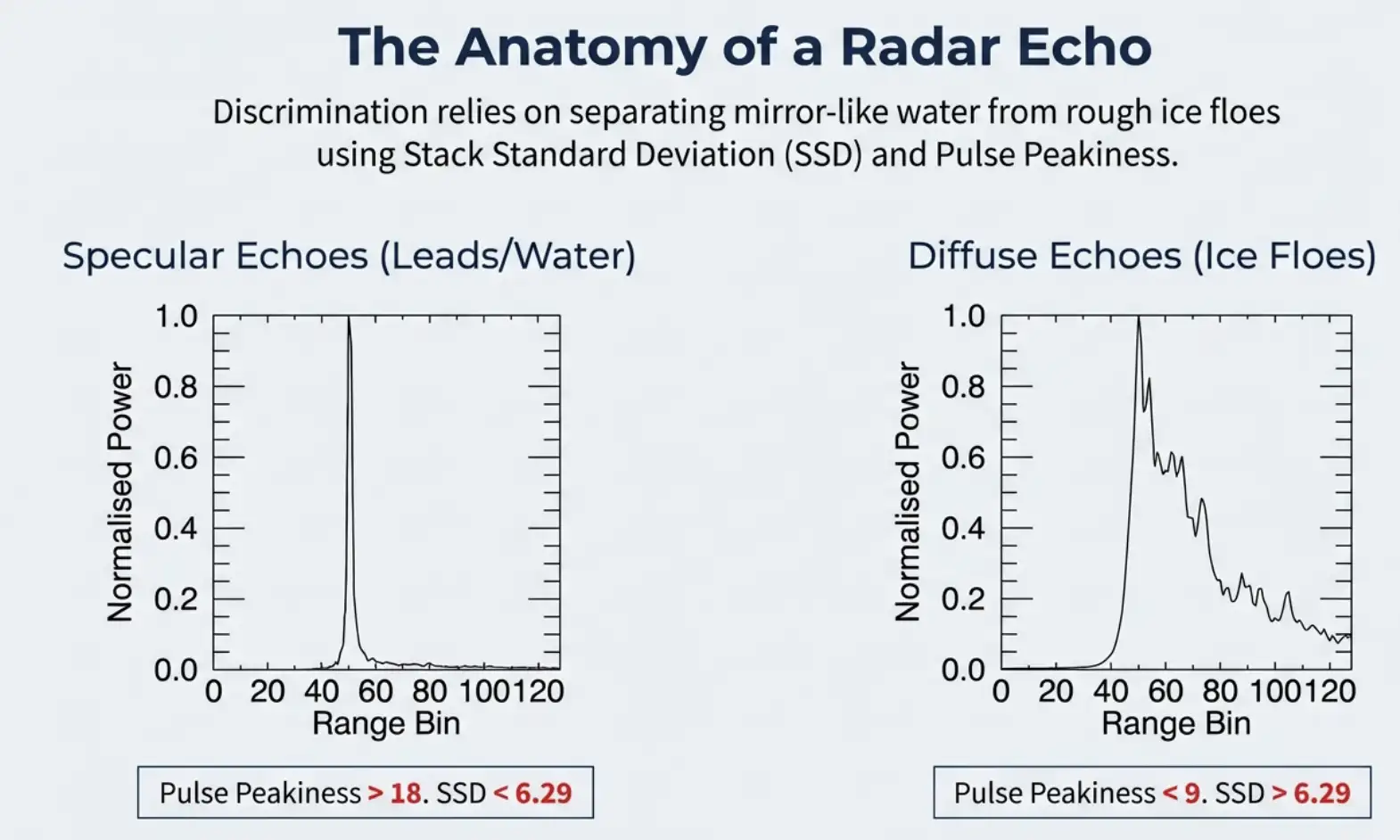
Incoming radar echoes are classified based on the shape of their individual pulse waveforms. Narrow, specular echoes are identified as originating from leads (cracks in the ice revealing the calm sea surface), while broader, diffuse echoes are classified as rougher sea ice floes.
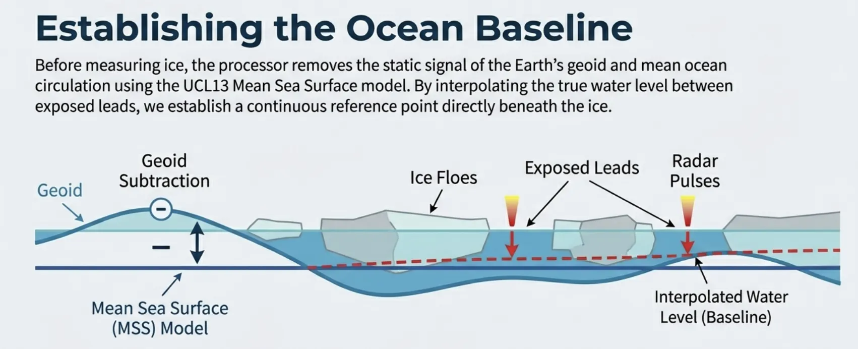
To calculate how high the ice sits above the water, we must first determine the 'local sea level' beneath the ice. We do this by comparing our lead elevations to a Mean Sea Surface (MSS) model (UCL13), which accounts for the permanent shape of the ocean. The difference between the measured lead height and the MSS is the Sea Level Anomaly (SLA), caused by tides and atmospheric pressure. We interpolate these SLA values across the ice floes to establish a continuous 'zero-level' sea surface, allowing us to isolate the ice freeboard from the ocean's background topography.
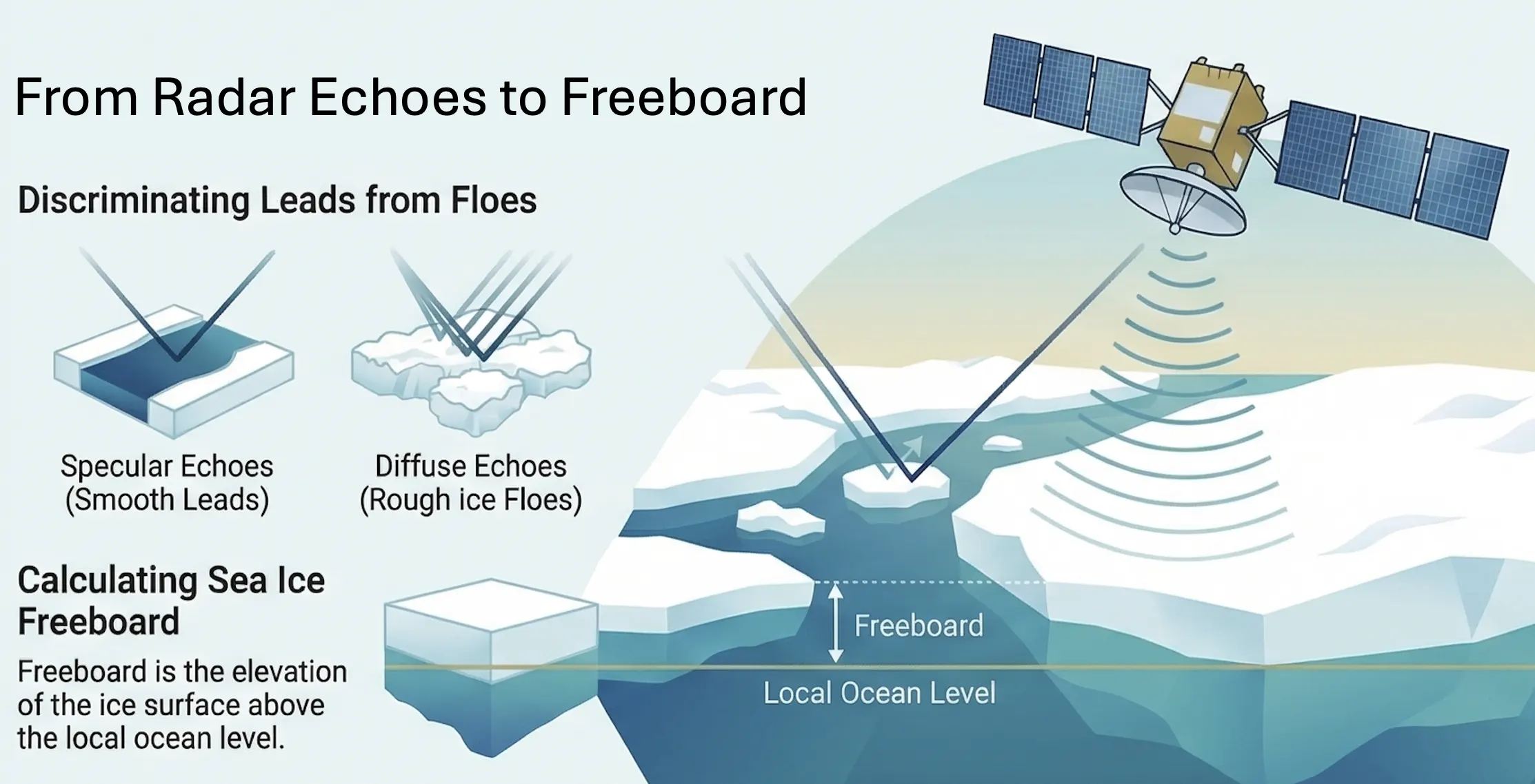
By isolating the elevation of the leads, a localized Sea Surface Height (SSH) is interpolated. The radar freeboard is then calculated as the physical difference in elevation between the top of the snow/ice interface (the sea ice floes) and this continuously interpolated local sea surface.
Radar propagation speed is slower through snow than air, and the physical weight of snow pushes the ice deeper into the water. To correct for this, a modified Warren 1999 (W99) snow depth and density climatology is applied. To account for the thinner snowpack typical of modern multi-year ice depletion, the W99 depth is halved over regions identified as first-year ice.
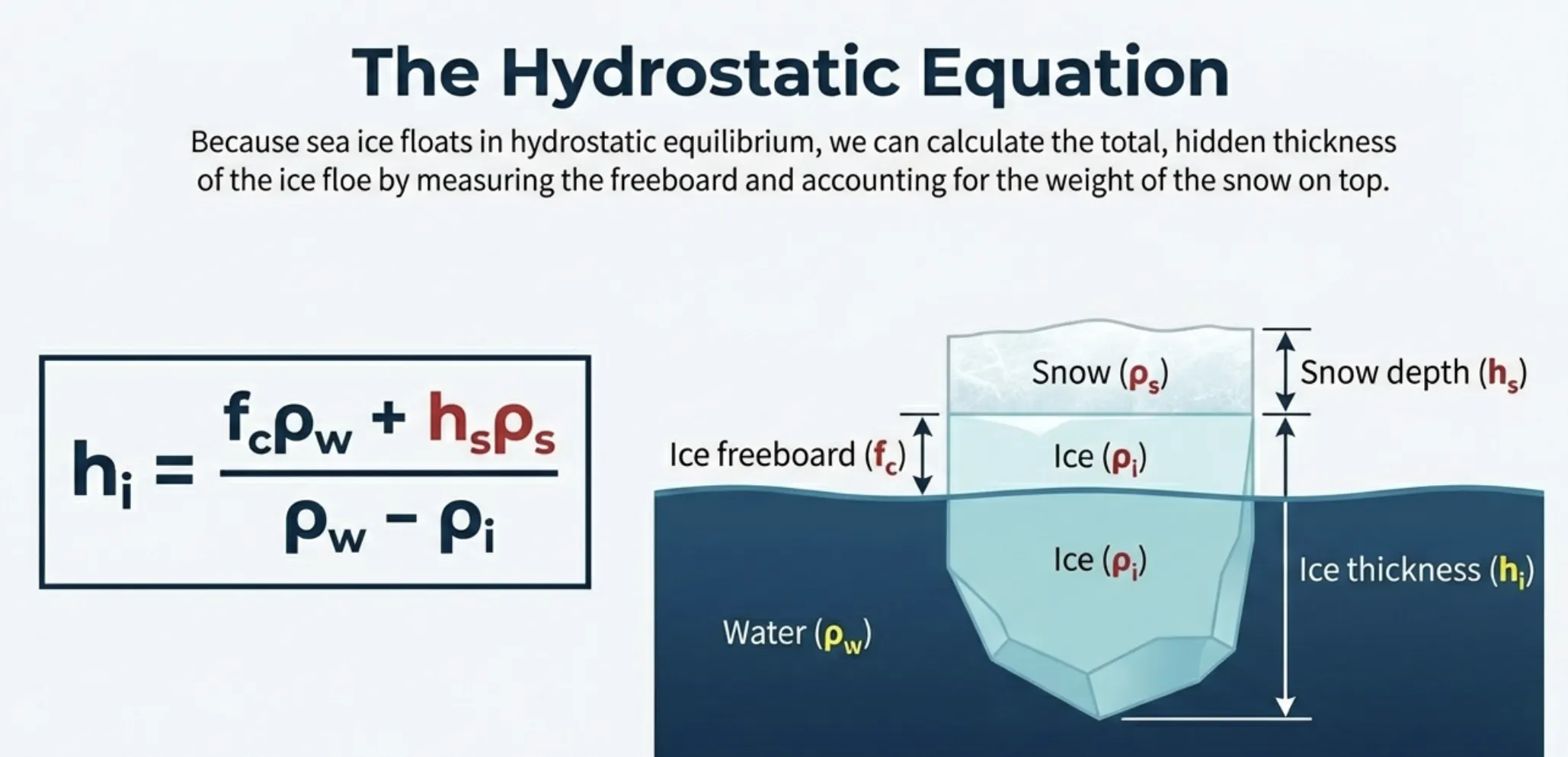
The corrected radar freeboard is converted into total sea ice thickness by assuming the ice floe represents a system in hydrostatic equilibrium. This calculation requires the constant densities of sea ice, snow, and seawater to model how much ice exists below the waterline based on the measured freeboard above it.
Finally, regional and basin-wide sea ice volume is derived by multiplying the calculated ice thickness by the fractional sea ice concentration (provided by external datasets such as the OSI SAF) and the corresponding geographic area of each grid cell.